Enter a Study on a Data Table
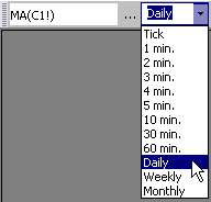
You may enter study syntax directly onto a data table, using the proper syntax and rules. The only difference in entering a study on a data table (vs. a quote) is that the aggregation is selected from the drop-down menu in the Active Plug-in toolbar, and not specified in the syntax. For information about entering study syntax onto a quote board or quote grid, go here.
CASE I - Simple One-Plot Studies
A one-plot study is one that draws only one line and displays one value on a chart.
-
Open a data table.
-
Select the desired aggregation from the drop-down list in the Active Plug-in toolbar.
-
With your cursor positioned in the Symbol field, enter the desired study syntax and press Enter:
function (source, value)

Examples:
|
MA('C 1!')
|
Shows a Moving Average on C 1! using default study parameter values.
|
|
=MA('C 1!', 10)
|
Shows a Moving Average on C 1!, using an overridden study parameter value of 10.
|
|
DMA('W 1!')
|
Shows a Displaced Moving Average on W 1! using default study parameter values.
|
|
=DMA('W 1!', 10, 14)
|
Shows a Displaced Moving Average on W 1! using overridden study parameter values of 10 and 14.
|
|
DMA('W 1!'.CLOSE)
|
Calculates a Displaced Moving Average on W 1! using the Input Field Close (vs the default input field). Uses default study parameters.
|
CASE II - Study Expressions
An expression is any mathematical calculation. Expressions may contain function names of studies. You may string together multiple expressions with the pipe operator " | ".
-
Open a data table.
-
Select the desired aggregation from the drop-down list in the Active Plug-in toolbar.
-
With your cursor positioned in the Symbol cell, enter the desired study syntax and press Enter:
Examples:
|
=0.5*(EMA('IN A0') + MA('IN A0'))
|
Adds the values of an SPY Exponential Moving Average and the SPY Moving Average, and multiplies the sum by 0.5
|
|
=(OSC('C 1!') + OSC('C 2!') + OSC('C 3!'))/3
|
Adds an Oscillator for the front month and next two months for Corn, then divides the result by 3.
|
|
=(RSI('ES 1!', 18) + TRIX('SP 1!', 12))
|
Adds the value of RSI calculated on ES1! (using an overridden parameter value of 18) with the value of TRIX calculated on SP1! (using an overridden parameter value of 12)
|
|
MA('ES 1!')|MA('ES 2!')|MA('SP 1!')|MA('SP 2!')
|
Displays 4 Moving Averages on the symbols ES1!, ES2!, SP1!, SP2!
|
CASE III - Multiple-Plot Studies
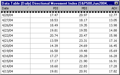
A multiple-plot study is one that draws more than one line and displays more than one value on a chart. Some examples of multiple-plot studies are Bollinger Bands, Directional Movement Index, Envelope, Line Oscillator, and MACD. The example below is the DMI, showing all three plots.

-
Open a data table.
-
Select the desired aggregation from the drop-down list in the Active Plug-in toolbar.
-
With your cursor positioned in the Symbol cell, enter the desired study syntax and press Enter. Multiple plot studies will display columns for all plots entered. For a list of Plot Names, please see the Function Names list.
function (source.InputField, value, value, value)
Examples:
|
DMI('SP 1!')
|
Calculates all three plots for the DMI on symbol SP1!
|
|
=DMI('SP 1!', HIGH, LOW, OPEN, 18)
|
Calculates all three plots for the DMI on symbol SP1!, overriding the study parameters.
|
|
BOLL('IN A0')
|
Calculates all three plots for the Bollinger Bands on symbol SPY.
|
|
=BOLL('IN A0', 12, 3)
|
Calculates all three plots for the Bollinger Bands on symbol SPY, overriding the study parameters.
|

